Tutorial: Raster-scan simulations - Thermoplasmonics

01/2021: updated to pyGDM v1.1+

This is an example how to simulate raster-scans in pyGDM.

We start again by loading the pyGDM modules that we are going to use:

import numpy as np
import matplotlib.pyplot as plt

from pyGDM2 import structures
from pyGDM2 import materials
from pyGDM2 import fields
from pyGDM2 import propagators

from pyGDM2 import core
from pyGDM2 import linear
from pyGDM2 import nonlinear
from pyGDM2 import visu
from pyGDM2 import tools

Simulation setup

We’ll use water as environment (n=1.33, kappa=0.6 W (m^-1 K^1) )

## --- Setup structure
step = 20.0
geometry = structures.rhombus(step, L=int(520/step), H=1, alpha=60, mesh='hex')
geometry = structures.center_struct(geometry)
material = materials.gold()
struct = structures.struct(step, geometry, material)


## --- Setup incident field
field_generator = fields.focused_planewave        # planwave excitation

## 50nm spotsize: LDOS; 200nm spotsize: TPL map
kwargs = dict(theta = [0, 90], spotsize=[200], kSign=-1,
              xSpot=np.linspace(-500, 500, 25),
              ySpot=np.linspace(-500, 500, 25))
wavelengths = [750]
efield = fields.efield(field_generator, wavelengths=wavelengths, kwargs=kwargs)


## --- homogeneous environment: water
n1, n2 = 1.33, 1.33  # constant environment (water)
dyads = propagators.DyadsQuasistatic123(n1=n1, n2=n2)


## ---------- Simulation initialization
sim = core.simulation(struct, efield, dyads)

structure initialization - automatic mesh detection: hex
structure initialization - consistency check: 676/676 dipoles valid

Let’s see what we configured there. First we plot an XY projection of the structure, then we will see what raster-scan configurations we get from the above defined field-parameters (kwargs):

## --- plot the structure
visu.structure(sim.struct.geometry, scale=0.5)
print("N dipoles:", len(sim.struct.geometry))

## --- for info: get a list of all raster-scan map configurations defined in "sim"
rasterscan_fieldconfigs = tools.get_possible_field_params_rasterscan(sim)
print('\n\n --- available rasterscan configurations:')
for i, p in enumerate(rasterscan_fieldconfigs):
    print("index {}: {}".format(i, p))

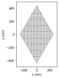
N dipoles: 676


 --- available rasterscan configurations:
index 0: {'kSign': -1, 'spotsize': 200, 'theta': 0, 'wavelength': 750}
index 1: {'kSign': -1, 'spotsize': 200, 'theta': 90, 'wavelength': 750}

• Indices “0” and “1” correspond to two full rasterscans with perpendicular polarizations of the incident field

Let’s run the simulation:

sim.scatter()

/home/hans/.local/lib/python3.8/site-packages/numba/core/dispatcher.py:237: UserWarning: Numba extension module 'numba_scipy' failed to load due to 'ValueError(No function '__pyx_fuse_0pdtr' found in __pyx_capi__ of 'scipy.special.cython_special')'.
  entrypoints.init_all()

timing for wl=750.00nm - setup: EE 11288.8ms, inv.: 395.6ms,

/home/hans/.local/lib/python3.8/site-packages/pyGDM2/fields.py:1309: UserWarning: `focuses_planewave` is deprecated. It is recommended to using `gaussian` instead .
  warnings.warn("`focuses_planewave` is deprecated. " +
/home/hans/.local/lib/python3.8/site-packages/pyGDM2/fields.py:1184: UserWarning: `planewave` is deprecated and supports only normal incidence/homogeneous environments. It is recommended to using `plane_wave` instead (with underscore in function name).
  warnings.warn("`planewave` is deprecated and supports only normal incidence/homogeneous environments. " +
/home/hans/.local/lib/python3.8/site-packages/pyGDM2/fields.py:1309: UserWarning: `focuses_planewave` is deprecated. It is recommended to using `gaussian` instead .
  warnings.warn("`focuses_planewave` is deprecated. " +
/home/hans/.local/lib/python3.8/site-packages/pyGDM2/fields.py:1184: UserWarning: `planewave` is deprecated and supports only normal incidence/homogeneous environments. It is recommended to using `plane_wave` instead (with underscore in function name).
  warnings.warn("`planewave` is deprecated and supports only normal incidence/homogeneous environments. " +

repropa.: 6767.3ms (1250 field configs), tot: 18451.9ms

1

Note that core.scatter above calculated \(2 \times 25 \times 25 = 1250\) simulations!

Calcuate raster-scan maps

Now comes the part where we calculate the raster-scan maps from the 1250 fields inside the nanoparticles (which are all stored in sim.E):

## raster-scan indices 0,1: 0,90 deg

## --- TPL
print("calculating TPL...")
TPL0 = tools.calculate_rasterscan(sim, 0, nonlinear.tpl_ldos)
TPL90 = tools.calculate_rasterscan(sim, 1, nonlinear.tpl_ldos)


## --- heat
print("calculating heat...")
Q0 = tools.calculate_rasterscan(sim, 0, linear.heat, return_units='uW')
Q90 = tools.calculate_rasterscan(sim, 1, linear.heat, return_units='uW')


## --- temperature increase
print("calculating temperature rise at (0,0,150)...")
r_probe = (0, 0, 150)
DT0 = tools.calculate_rasterscan(sim, 0, linear.temperature, r_probe=r_probe, kappa_env=0.6)
DT90 = tools.calculate_rasterscan(sim, 1, linear.temperature, r_probe=r_probe, kappa_env=0.6)

calculating TPL...
calculating heat...

/home/hans/.local/lib/python3.8/site-packages/pyGDM2/linear.py:1320: UserWarning: `linear_py.heat` does not support tensorial permittivity yet.
  warnings.warn("`linear_py.heat` does not support tensorial permittivity yet.")

calculating temperature rise at (0,0,150)...

Note: You should be sure to have chosen the correct indices (0 or 1 in our example) for the raster-scan simulations. That’s why we checked the indices above.

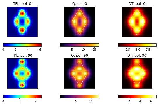
Plotting the maps

Now we have calculated 2D scalar maps of different physical quantities as function of a focused beam’s position on the structure. We need to do nothing more that plotting it:

plt.figure(figsize=(10,6))

## --- limit the number of ticks on the axes (for the colorbar!)
from matplotlib.ticker import MaxNLocator
MaxNLocator.default_params['nbins'] = 4


## --- TPL
plt.subplot(2,3,1, aspect='equal')
plt.xticks([]); plt.yticks([]); plt.title("TPL, pol. 0")
im = visu.scalarfield(TPL0, cmap='jet', show=False)
plt.colorbar(im, orientation='horizontal', shrink=0.8, aspect=12)
visu.structure_contour(geometry, color='w', dashes=[2,2], lw=1.0, show=0)

plt.subplot(2,3,4, aspect='equal')
plt.xticks([]); plt.yticks([]); plt.title("TPL, pol. 90")
im = visu.scalarfield(TPL90, cmap='jet', show=False)
plt.colorbar(im, orientation='horizontal', shrink=0.8, aspect=12)
visu.structure_contour(geometry, color='w', dashes=[2,2], lw=1.0, show=0)


## --- heat
plt.subplot(2,3,2, aspect='equal')
plt.xticks([]); plt.yticks([]); plt.title("Q, pol. 0")
im = visu.scalarfield(Q0, cmap='inferno', show=False)
plt.colorbar(im, orientation='horizontal', shrink=0.8, aspect=12)
visu.structure_contour(geometry, color='w', dashes=[2,2], lw=1.0, show=0)

plt.subplot(2,3,5, aspect='equal')
plt.xticks([]); plt.yticks([]); plt.title("Q, pol. 90")
im = visu.scalarfield(Q90, cmap='inferno', show=False)
plt.colorbar(im, orientation='horizontal', shrink=0.8, aspect=12)
visu.structure_contour(geometry, color='w', dashes=[2,2], lw=1.0, show=0)


## --- temperature rise
plt.subplot(2,3,3, aspect='equal')
plt.xticks([]); plt.yticks([]); plt.title("DT, pol. 0")
im = visu.scalarfield(DT0, cmap='hot', show=False)
plt.colorbar(im, orientation='horizontal', shrink=0.8, aspect=12)
visu.structure_contour(geometry, color='w', dashes=[2,2], lw=1.0, show=0)

plt.subplot(2,3,6, aspect='equal')
plt.xticks([]); plt.yticks([]); plt.title("DT, pol. 90")
im = visu.scalarfield(DT90, cmap='hot', show=False)
plt.colorbar(im, orientation='horizontal', shrink=0.8, aspect=12)
visu.structure_contour(geometry, color='w', dashes=[2,2], lw=1.0, show=0)


plt.show()