Here we give an overview of the pygdmUI package, a graphical user interface to pyGDM2.
Note: pygdmUI requires minimum pyGDM2 version v1.1.
pygdm-UI
pyGDM-UI is a pyqt based, pure python graphical user interface to pyGDM2. It provides the most common functionalities of pyGDM2 for rapid simulations and testing.
Requirements
Installation
Via pip
Install from pypi repository via
$ pip install pygdmUI
Manual
Download the latest code from gitlab or clone the git repository:
$ git clone https://gitlab.com/wiechapeter/pygdm-ui.git
$ cd pygdm-ui
$ python setup.py install --user
Run pyGDM-UI
In the terminal:
$ python3 -m pygdmUI.main
Overview
Structure compositor
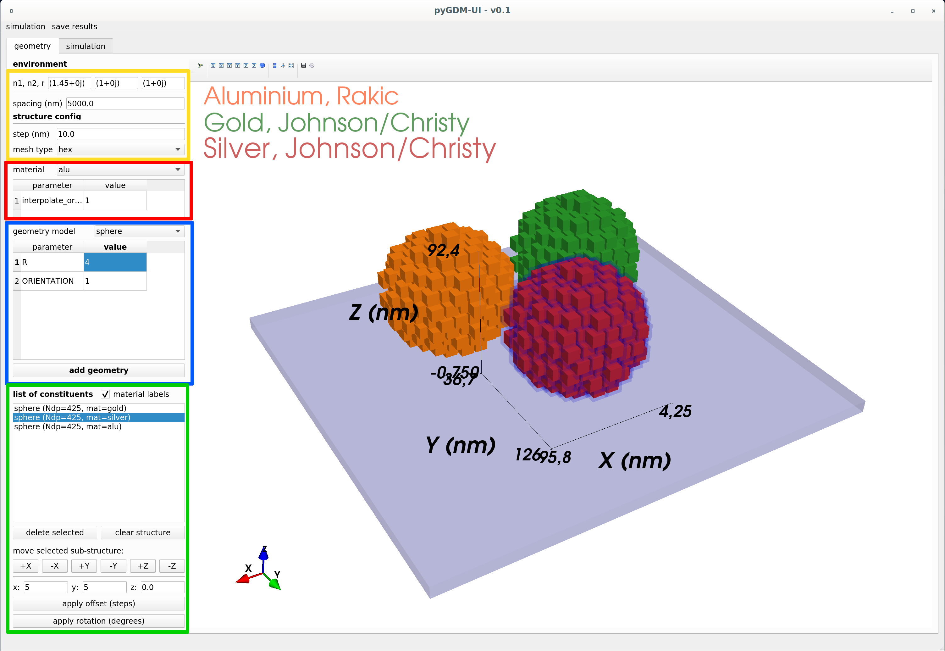
The first tab of the GUI is dedicated to compose a nanostructure, shown in the screenshot below. The yellow highlighted part configures the simulation environment, stepsize and mesh-type. The latter two parameters must be the same for all substructures. The red and blue areas are used to define the material (red box) and structure geometry (blue box) of a constituent of the nanostructure. The full structure can be then composed of different sub-geometries, which again can be of different material. The list of sub-geometries is show at the bottom (green highlighed box), where the individual sub-structures can also be moved around and rotated.
Simulation configurator
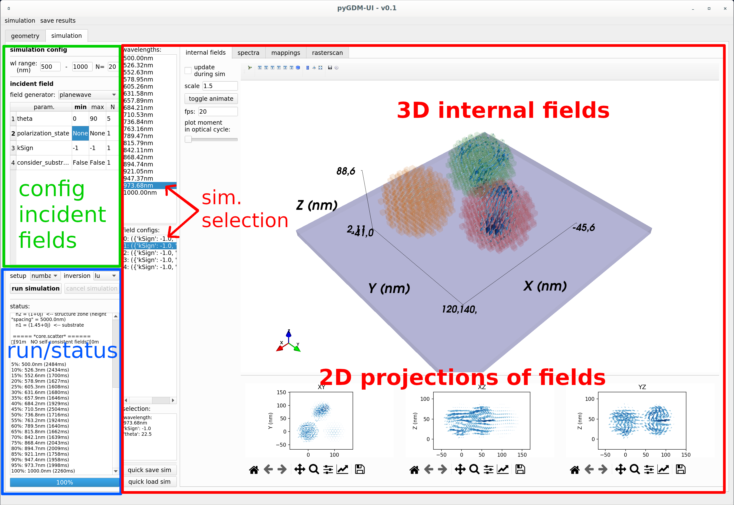
In the second tab of the GUI, incident field and it’s configurations are defined (green highlighted area). The wavelength range of the simulation is specified (a single wavelength can be achieved by setting N=1, in which case just the first wavelength will be used. The simulation is launched with the according button in the blue highlighted area, after chosing the solver (“setup” and “inversion”). This part of the GUI also contains a view of the internal electric fields, calculated in the simulation (red highlighted area). Furthermore, several tabs are available to analyze and visualize the results (spectra / mappings / rasterscan).
Simulation evaluation
Next to the view of the internal fields, further analysis and visualization of the results can be performed.
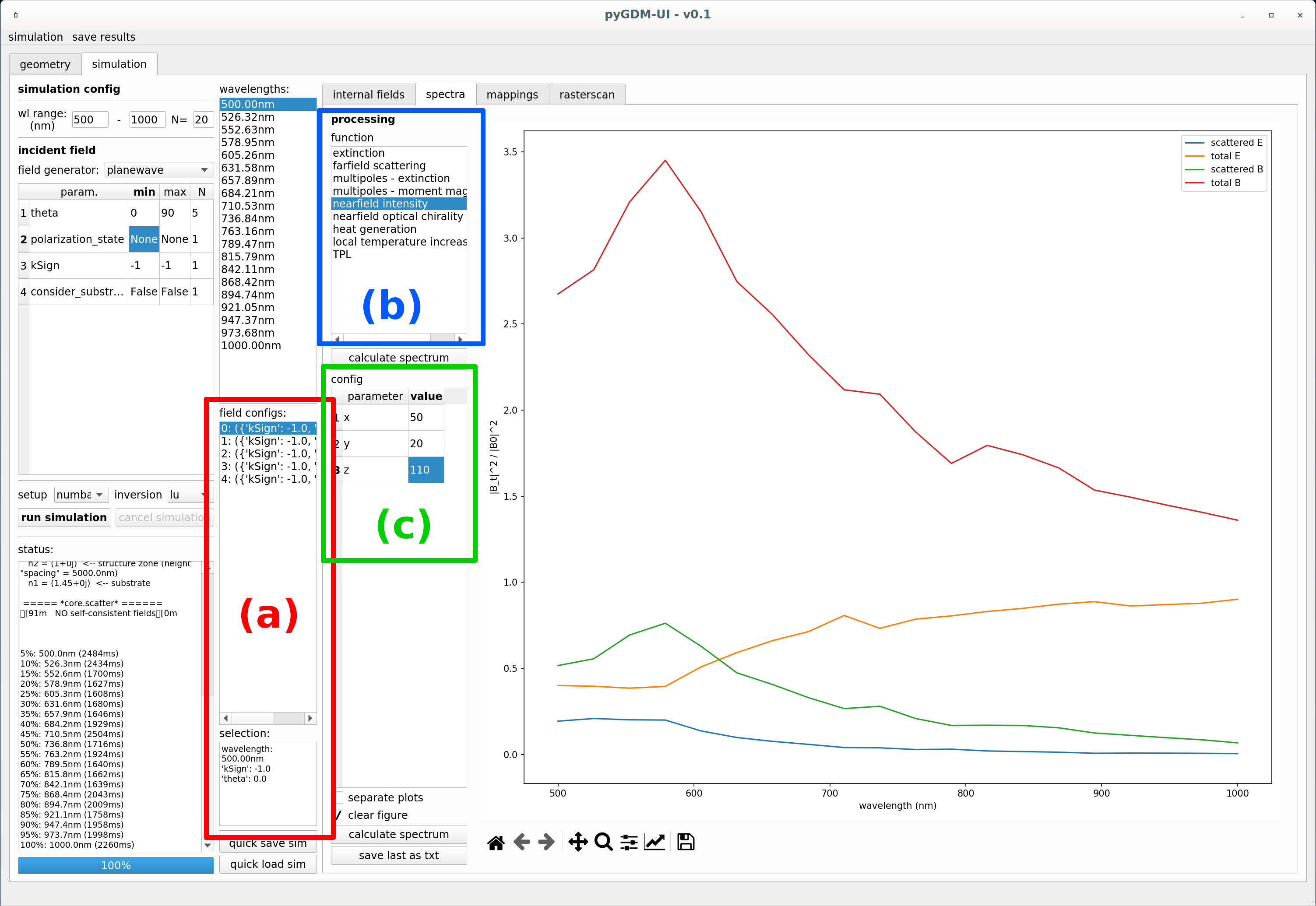
Spectra
In the “spectra” tab, a spectrum can be calculated, provided the simulation contains more than one wavelength. To do so, first a incident field configuration needs to be selected (red highlighted area (a) in the screenshot below). The spectrum will be calculated using these incident field parameters. Now, we chose the evaluation function (blue area (b)), in the example we want to calculate the spectrum of the nearfield intensity at a specific position. Finally, we need to configure the evaluation function. The available parameters are shown in the “config” section ((c), highlighted green). Finally, we launch the calculation by clicking on one of the “calculate spectrum” buttons.
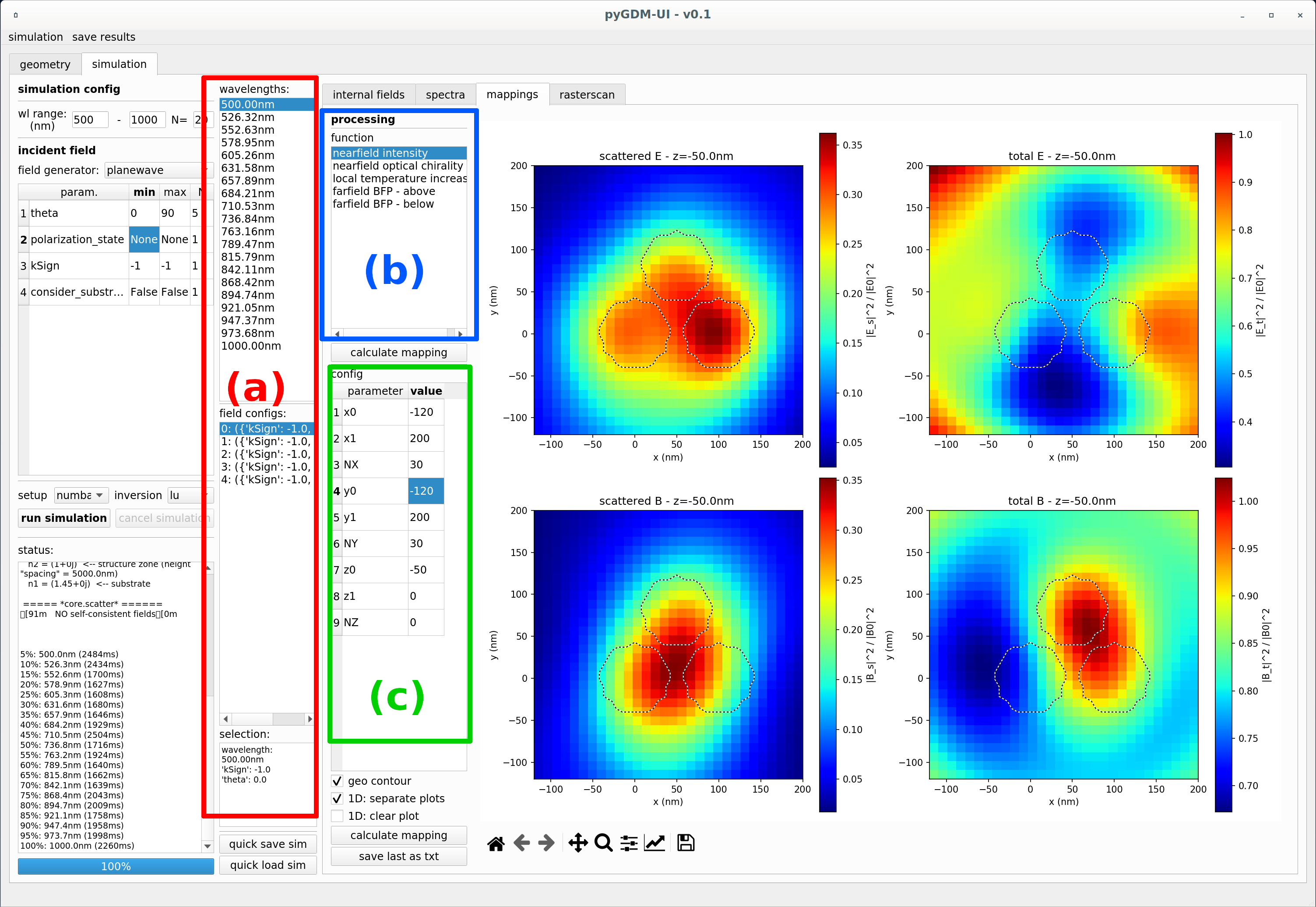
Spatial profiles / mappings
A second possibility is to post-process the results at a specific incident wavelength and field configuration. These can be done in the “mappings” tab, either along 1D line-profiles or on 2D mappings. For instance, we can evaluate the nearfield intensity on a 2D mapping, as shown in the below example (for a 1D line-profile, set NX=0 or NY=0, the position x0, respectively y0, will then be used).
First, select a wavelength and a field-configuration (like polarization, etc…) in the according lists (a), highlighted red in the screenshot below. Then, select an evluation function in the list (b) (blue). Finally, enter the configuration for the evaluation function in the green highlighed table (c), which is in case of the nearfield intensity simply the mapping dimensions and number of steps. After clicking “calculate mapping”, the evaluation is launched and, once finished, the results are displayed on the right.
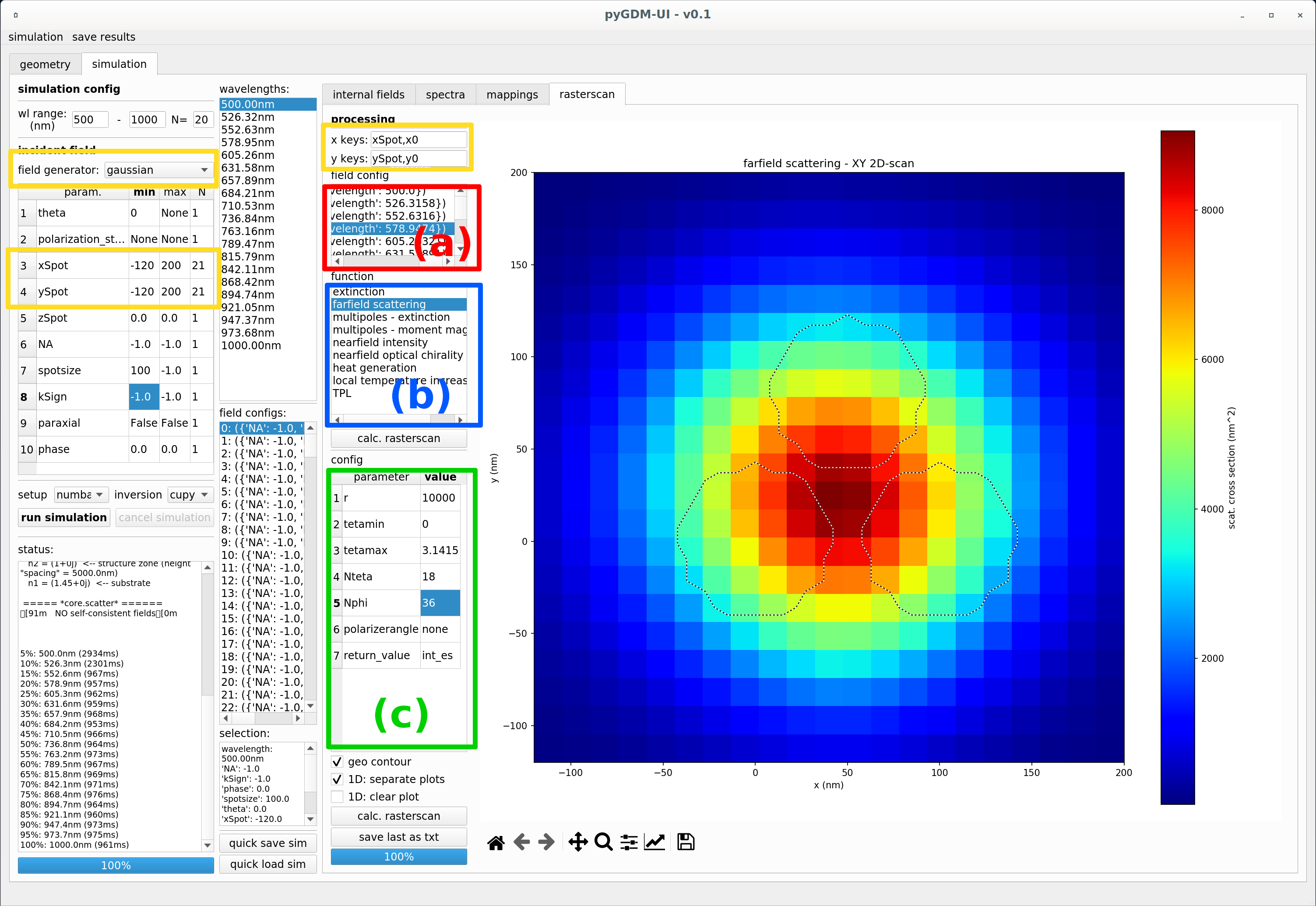
Raster-scan simulations
A great advantage of the GDM is the possibility to calculate rasterscan simulations very efficiently, since the entire scattering problem is solved by calculation of the generalized propagator. A rasterscan simulation requires of course an incident field which is raster-scanned across the nanostructure. This can be a focused beam like the gaussian incident field below, but also a dipole emitter. In the below example, we first configure a raster-scanned incident field (yellow highlighted areas). The evaluation routine will search for keywords as defined by the (comma separated) “x keys” and “y keys” fields, so these need to contain the appropriate scan parameters. By adapting those fields, also a z-scan can be performed (scanning for instance a dipole emitter).
In the example we use a Gaussian beam and a 2D rasterscan area, but is is also possible to use a 1D-scanning path. pygdmUI will then plot 1D figures upon evaluation. We first chose the field configuration (e.g. wavelength, polarization, …) in the red highlighed area (a). In the list (b) surrounded by a blue line, we then select again an evaluation function, which will be called at each incident field scanning position. In the below example we shall calculate far-field scattering, integrated over a full sphere at 10 microns radius around the nanostructure, this configuration is done in the “config” table (c), highlighted with a green frame.