Tutorial: Field-maps

01/2021: updated to pyGDM v1.1+

This is an example how to calculate the electric and magnetic field outside the nano-structure.

from pyGDM2 import core
from pyGDM2 import propagators
from pyGDM2 import structures
from pyGDM2 import materials
from pyGDM2 import fields
from pyGDM2 import linear
from pyGDM2 import tools
from pyGDM2 import visu

import matplotlib.pyplot as plt

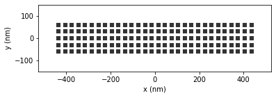
Simulation: Silicon nanowire

We will setup a simulation for a cuboidal silicon nanowire, evaluated at a single wavelength and linear polarization. For the polarization angle we will use an angle somewhat off the nanowire long axis:

## ---------- Setup structure
mesh = 'cube'
step = 30.0
geometry = structures.rect_wire(step, L=30,H=4,W=5, mesh='cube')
geometry = structures.center_struct(geometry)
material = materials.silicon()

struct = structures.struct(step, geometry, material)


## ---------- Setup incident field
field_generator = fields.plane_wave
kwargs = dict(theta = [30.0])  ## by default: incidence from top
wavelengths = [600]
efield = fields.efield(field_generator, wavelengths=wavelengths, kwargs=kwargs)


## ---------- vacuum environment
n1 = n2 = 1.0
dyads = propagators.DyadsQuasistatic123(n1=n1, n2=n2)


## ---------- Simulation initialization
sim = core.simulation(struct, efield, dyads)

print("N dipoles:", len(sim.struct.geometry))
visu.structure(geometry, scale=0.7)

#==============================================================================
# run the simulation: possible either via sim.scatter() or via core.scatter(sim)
#==============================================================================
E = core.scatter(sim)

structure initialization - automatic mesh detection: cube
structure initialization - consistency check: 600/600 dipoles valid
N dipoles: 600

/home/hans/.local/lib/python3.8/site-packages/pyGDM2/visu.py:49: UserWarning: 3D data. Falling back to XY projection...
  warnings.warn("3D data. Falling back to XY projection...")

/home/hans/.local/lib/python3.8/site-packages/numba/core/dispatcher.py:237: UserWarning: Numba extension module 'numba_scipy' failed to load due to 'ValueError(No function '__pyx_fuse_0pdtr' found in __pyx_capi__ of 'scipy.special.cython_special')'.
  entrypoints.init_all()

timing for wl=600.00nm - setup: EE 10720.7ms, inv.: 282.5ms, repropa.: 8047.2ms (1 field configs), tot: 19050.8ms

OK, now we need to calculate field-maps outside the structure ————————————————–

We will do several field-maps at increasing distances from the nanowire and compare those.

#==============================================================================
# Nearfield map below structure
#==============================================================================
distances = [-1*step, -3*step, -5*step, -7*step]

Es = []
Bs = []
Etot = []
Btot = []
for Z0 in distances:
    r_probe = tools.generate_NF_map_XY(-500,500,51, -500,500,51, Z0=Z0)

    ## --- linear.nearfield takes either a whole "map" or only a
    ## --- 3D coordinate as input. Here we want the field on a map.
    _Es, _Etot, _Bs, _Btot = linear.nearfield(sim, field_index=0, r_probe=r_probe)
    Es.append(_Es)
    Etot.append(_Etot)
    Bs.append(_Bs)
    Btot.append(_Btot)

Using the visu module, we plot the fields as 2D vector representation as well as the field-intensity as colorplot.

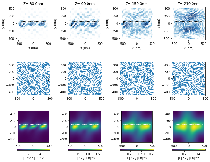
Scattered electric field

## --- limit the number of ticks on the axes (for the colorbar!)
from matplotlib.ticker import MaxNLocator
MaxNLocator.default_params['nbins'] = 4

## the plot
plt.figure(figsize=(10, 8))

for i, _Es in enumerate(Es):
    ## --- field vectors
    plt.subplot(3,len(Es),1+i, aspect='equal')
    plt.title("Z={}nm".format(distances[i]))
    visu.structure_contour(sim, zorder=10, dashes=[2,2], color='k', show=0)
    visu.vectorfield(_Es, show=0, EACHN=2)

    ## --- field isolines
    plt.subplot(3,len(Es),1+1*len(Es)+i, aspect='equal')
    visu.structure_contour(sim, zorder=10, dashes=[2,2], color='k', show=0)
    visu.vectorfield_fieldlines(_Es, show=0)

    ## --- field intensity
    plt.subplot(3,len(Es),1+2*len(Es)+i, aspect='equal')
    visu.structure_contour(sim, zorder=10, dashes=[2,2], color='w', show=0)
    im = visu.vectorfield_color(_Es, show=0)
    plt.colorbar(im, orientation='horizontal', label="|E|^2 / |E0|^2")

plt.tight_layout()
plt.show()

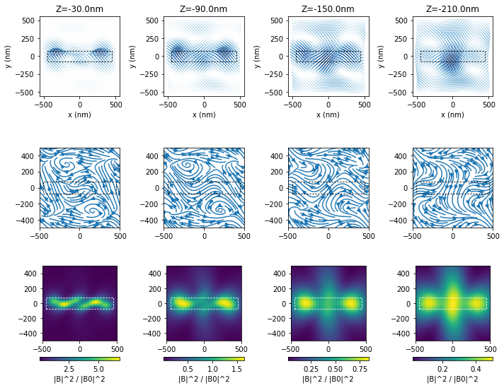
Scattered magnetic field

plt.figure(figsize=(10, 8))

for i, _Bs in enumerate(Bs):
    ## --- field vectors
    plt.subplot(3,len(Bs),1+i, aspect='equal')
    plt.title("Z={}nm".format(distances[i]))
    visu.structure_contour(sim, zorder=10, dashes=[2,2], color='k', show=0)
    visu.vectorfield(_Bs, show=0, EACHN=2)

    ## --- field isolines
    plt.subplot(3,len(Bs),1+1*len(Bs)+i, aspect='equal')
    visu.structure_contour(sim, zorder=10, dashes=[2,2], color='k', show=0)
    visu.vectorfield_fieldlines(_Bs, show=0)

    ## --- field intensity
    plt.subplot(3,len(Bs),1+2*len(Bs)+i, aspect='equal')
    visu.structure_contour(sim, zorder=10, dashes=[2,2], color='w', show=0)
    im = visu.vectorfield_color(_Bs, show=0)
    plt.colorbar(im, orientation='horizontal', label="|B|^2 / |B0|^2")

plt.tight_layout()
plt.show()