Here we give a short survey of what pyGDM does and of the underlying approximations of some of the main functionalities.
Overview
pyGDM is based on the Green Dyadic Method (GDM) which resolves an optical Lippmann-Schwinger equation and calculates the total electromagnetic field \(\big \{\mathbf{E}(\mathbf{r}, \omega),\mathbf{H}(\mathbf{r}, \omega)\big \}\) , inside a nanostructure, embedded in a fixed environment, upon illumination by an incident electromagnetic field \(\big \{\mathbf{E}_0(\mathbf{r}, \omega),\mathbf{H}_0(\mathbf{r}, \omega)\big \}\). The environment is described by the Green’s tensors \(\mathbf{G}^{\text{EE}}_{\text{tot}}(\mathbf{r}, \mathbf{r'}, \omega)\) and \(\mathbf{G}^{\text{HE}}_{\text{tot}}(\mathbf{r}, \mathbf{r'}, \omega)\):
GDM is a frequency-domain method, hence the fields are required to be monochromatic and time-harmonic. From the complex electromagnetic fields inside the nanostructure, further physical quantities can be derived such as local fields outside the nanostructure, far-field scattering and extinction cross-sections or radiation patterns and local heat generation. It is also possible to calculate local densities of photonic states and hence the decay rates of quantum emitters close to the structure.
Volume discretization
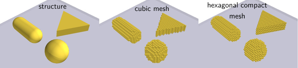
The GDM is a volume integral equation approach. The volume integration runs over the nanostructure. It is numerically implemented as a discretization of the structure volume on a regular mesh. This discretization turns the integral over the nanostructure volume into a sum of all N mesh cells with volume \(V_{\text{cell}}\). This transforms the Lippmann-Schwinger equations into a system of coupled equations, that can be resolved by matrix inversion:
In pyGDM, the discretization is done either on a cubic grid (center panel in image below), or on a hexagonal compact grid (right panel in image below).
Simulation environment
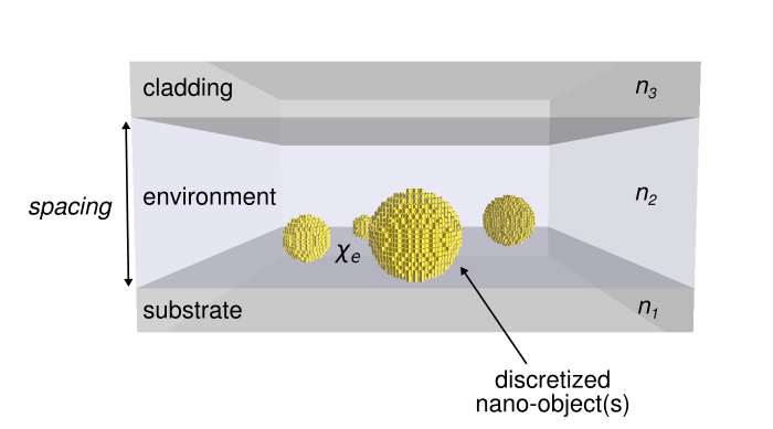
One advantage of GDM compared to domain discretization techniques such as FDTD is that only the nanostructure is discretized. The environment in which the nanostructure is embedded is described by the Green’s dyadic functions \(\mathbf{G}^{\text{EE}}_{\text{tot}}(\mathbf{r}, \mathbf{r'}, \omega)\) and \(\mathbf{G}^{\text{HE}}_{\text{tot}}(\mathbf{r}, \mathbf{r'}, \omega)\), used in the calculation. As shown in the below figure, pyGDM implements a Green’s dyad for a 3-layer environmental frame, the nanostructure itself lying in the center layer.
The below code example shows how to implement the environment since the version 1.1 of pyGDM. The class propagators contains the differents Green’s tensors. The choice of the tensor depends of the nature of the problem (“2D” or “3D”) and the refractive index of the environments “n1”, “n2” and “n3”.
## now we setup the class of Greens tensors (Dyads) defining the environment
    ## n1: substrate refractive index
    ## n2: top environment index
    n1, n2 = 1, 1
    dyads = propagators.DyadsQuasistatic123(n1=n1, n2=n2)


    .. rst-class:: html-toggle
Mathematical definitions of \(\mathbf{G}^{\text{EE}}_{\text{tot}}(\mathbf{r}, \mathbf{r'}, \omega)\) and \(\mathbf{G}^{\text{HE}}_{\text{tot}}(\mathbf{r}, \mathbf{r'}, \omega)\)
The explicit definitions of the tensors \(\mathbf{G}^{\text{EE}}_{\text{tot}}(\mathbf{r}, \mathbf{r'}, \omega)\) and \(\mathbf{G}^{\text{HE}}_{\text{tot}}(\mathbf{r}, \mathbf{r'}, \omega)\) are fully summarized and explained in the paper “PyGDM New functionalities” https://arxiv.org/abs/2105.04587. A brief summary of the different terms is given below
3D case :
If n1=n2=n3
\[\begin{split}&\bullet\mathbf{G}^{\text{EE}}_{\text{tot}}(\mathbf{r}, \mathbf{r'}, \omega) = \mathbf{G}^{\text{EE}}_0(\mathbf{r}, \mathbf{r'}, \omega) \\ &\bullet\mathbf{G}^{\text{HE}}_{\text{tot}}(\mathbf{r}, \mathbf{r'}, \omega) = \mathbf{G}^{\text{HE}}_0(\mathbf{r}, \mathbf{r'}, \omega)\end{split}\]
with \(\mathbf{G}^{\text{EE}}_0(\mathbf{r}, \mathbf{r'}, \omega)\) and \(\mathbf{G}^{\text{HE}}_0(\mathbf{r}, \mathbf{r'}, \omega)\) the homogeneous field susceptibilities.
If n1 \(\neq\) n2 \(\neq\) n3
\[\begin{split}&\bullet\mathbf{G}^{\text{EE}}_{\text{tot}}(\mathbf{r}, \mathbf{r'}, \omega) = \mathbf{G}^{\text{EE}}_0(\mathbf{r}, \mathbf{r'}, \omega) + \mathbf{G}^{\text{EE}}_{\text{3-layer}}(\mathbf{r}, \mathbf{r'}, \omega) \\ &\bullet\mathbf{G}^{\text{HE}}_{\text{tot}}(\mathbf{r}, \mathbf{r'}, \omega) = \mathbf{G}^{\text{HE}}_0(\mathbf{r}, \mathbf{r'}, \omega)\end{split}\]
where \(\mathbf{G}^{\text{EE}}_{\text{3-layer}}(\mathbf{r}, \mathbf{r'}, \omega)\) is the field susceptibility associated with a substrate an/or cladding layer. By default, for computational efficiency, this tensor is based on a quasi-static approximation. Since the version 1.1, the retarded expression of this tensor is available in the pyGDM2_retard module.
If \(\mathbf{r}=\mathbf{r'}\)
A self-term \(\mathbf{G}^{\text{EE}}_0(\mathbf{r}, \mathbf{r}, \omega)\) must be added to the total susceptibility \(\mathbf{G}^{\text{EE}}_{\text{tot}}(\mathbf{r}, \mathbf{r'}, \omega)\). The self-term expression depends of the discretization grid
\[\begin{split}&\bullet\mathbf{G}^{\text{EE}}_{\text{0,cube}}(\mathbf{r}, \mathbf{r}, \omega) = \frac{4\pi}{3\epsilon_{\text{env}}d^3}\mathbf{I} \\ &\bullet\mathbf{G}^{\text{EE}}_{\text{0,hex}}(\mathbf{r}, \mathbf{r}, \omega) = \frac{4\pi\sqrt{2}}{3\epsilon_{\text{env}}d^3}\mathbf{I}\end{split}\]
where d is the discretization step and \(\epsilon_{\text{env}}\) the dielectric constant of the environment containing the dipole.
2D case :
For infinites structures along y, the expression of the “2D” tensors is deduced by integrating the “3D” tensors along the invariance axis y
\[\mathbf{G}_0^{2D,\text{EE}} ( \mathbf{r}^{2D}, \mathbf{r}'^{,2D} ) = \int\limits_{-\infty}^{\infty} \mathbf{G}_0^{\text{EE}} (\mathbf{r}, \mathbf{r}') e^{\text{i} k_{y,0} y'} \text{d}y'\]
where \(\mathbf{r}^{2D}=x\hat{e}_x + z\hat{e}_z\) is the radial position.
If n1=n2=n3
\[\begin{split}&\bullet\mathbf{G}^{\text{2D,EE}}_{\text{tot}}(\mathbf{r}, \mathbf{r'}, \omega) = \mathbf{G}^{\text{2D,EE}}_0(\mathbf{r}, \mathbf{r'}, \omega) \\ &\bullet\mathbf{G}^{\text{2D,HE}}_{\text{tot}}(\mathbf{r}, \mathbf{r'}, \omega) = \mathbf{G}^{\text{2D,HE}}_0(\mathbf{r}, \mathbf{r'}, \omega)\end{split}\]
with \(\mathbf{G}^{\text{2D,EE}}_0(\mathbf{r}, \mathbf{r'}, \omega)\) and \(\mathbf{G}^{\text{2D,HE}}_0(\mathbf{r}, \mathbf{r'}, \omega)\) the homogeneous field susceptibilities.
If n1 \(\neq\) n2 \(\neq\) n3
\[\begin{split}&\bullet\mathbf{G}^{\text{2D,EE}}_{\text{tot}}(\mathbf{r}, \mathbf{r'}, \omega) = \mathbf{G}^{\text{2D,EE}}_0(\mathbf{r}, \mathbf{r'}, \omega) + \mathbf{G}^{\text{EE}}_{\text{3-layer}}(\mathbf{r}, \mathbf{r'}, \omega) \\ &\bullet\mathbf{G}^{\text{2D,HE}}_{\text{tot}}(\mathbf{r}, \mathbf{r'}, \omega) = \mathbf{G}^{\text{2D,HE}}_0(\mathbf{r}, \mathbf{r'}, \omega)\end{split}\]
As for the “3D” case, a self-term must be added if \(\mathbf{r}=\mathbf{r'}\).
Note
In the quasi-static approximation, there is no contribution of the layered environment to the mixed field susceptibility. The retarded mixed field susceptibility, associated with the surface, is not yet implemented in pyGDM.
Fundamental fields
The Lippmann Schwinger equation self-consistently relates the zero order field \(\mathbf{E}_0(\mathbf{r}, \omega)\) (without presence of the nanostructure) and the field \(\mathbf{E}(\mathbf{r}, \omega)\) upon interaction of the field with the nanostructure. Hence, any incident field \(\mathbf{E}_0(\mathbf{r}, \omega)\) can be used to excite the nanostructure. Several illumination field generators are available in pyGDM, with the possibility to easily write custom extensions and own fields.
The below code example shows how to implement a plane wave fundamental illumination.
## --- we define the type of incident illumination (here a plane wave)
    field_generator = fields.plane_wave
    ## --- then the range of wavelengths
    wavelengths = np.linspace(400, 1000, 30)
    ## --- Finally, the characteristics of the incoming light
    ## --- such as polarisations and angles of incidence
    kwargs = dict(theta=[0, 45, 90], inc_angle=180)

    efield = fields.efield(field_generator,
                               wavelengths=wavelengths, kwargs=kwargs)
The class fields contains all the illumination fields. All field definitions are summarised in the two pyGDM publications https://arxiv.org/abs/1802.04071 and https://arxiv.org/abs/2105.04587, with all terms explained. Below is an overview of these.
Plane wave :
Focused plane wave :
Paraxial Gaussian beam :
Tightly focused Gaussian beam :
Dipolar emitter :
Electric
Magnetic
In the pyGDM update we implemented a few additional focused vectorbeams, following chapter 3.6 of the textbook of Novotny and Hecht https://doi.org/10.1017/CBO9780511813535. We now provide generator functions for doughnut beams with azimuthal and radial polarization as well as linearly polarized Hermite-Gauss beams.
For 2 or 3-layer environmental frame, the reflected and transmitted fields through interfaces, \(\mathbf{E}_\text{r}(\mathbf{r}, \omega)\) and \(\mathbf{E}_\text{t}(\mathbf{r}, \omega)\), must be added to the above fields, then the illumination field \(\mathbf{E}_0(\mathbf{r}, \omega)\) becomes
Coupled dipole simulation
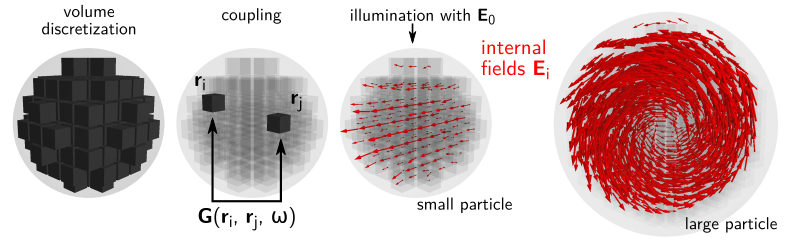
The main part of a pyGDM simulation is the calculation of the internal fields \(\mathbf{E}(\mathbf{r}, \omega)\) inside the nanostructure, by solving the discretized Lippmann Schwinger equation as given above. The matrix that defines this system of equations is determined by the Green’s Dyads \(\mathbf{G}(\mathbf{r}_i, \mathbf{r}_j, \omega)\), coupling all pairs of mesh-cells at \(\mathbf{r}_i\) and \(\mathbf{r}_j\) of the structure.
pyGDM, uses a near-field approximation of the Green’s Dyad for a layered system of 3 layers, which can be derived through the method of mirror charges. Hence, the approximation assumes that every mesh-point induces a mirror dipole in the substrate as well as in the cladding layer. This approximation is valid in the near-field region, when retardation effects can be neglected.
Post processing functions to derive physical quantities
As the illumination fields, the physical quantities obtained from the local electric field are fully developped in the two pyGDM papers https://arxiv.org/abs/1802.04071 and https://arxiv.org/abs/2105.04587 . A non-exhaustive list of the main equations is summarised here.
Detailed descriptions of the following quantities can be found in the paper https://arxiv.org/abs/1802.04071:
Extinction :
Absorption :
Scattering :
Note
The equations of \(\sigma_{\text{ext}}(\omega)\) and \(\sigma_{\text{abs}}(\omega)\) are not the same as in the article. These, with the refractive index of the environment \(n_{\text{env}}\) in the denominator, allow the modelling of non-vacuum media.
Farfield :
where \(\mathbf{G}^{\text{EE}}_{\text{ff}}(\mathbf{r}_j, \mathbf{r})\) is the asymptotic expression of \(\mathbf{G}^{\text{EE}}_{\text{tot}}\). This asymptotic tensor is fully developped, in the second article on pyGDM https://arxiv.org/abs/2105.04587, for homogenenous and 2-layer media.
Heat :
Temperature :
TPL :
Decay rates :
Electric dipole
Magnetic dipole
Detailed descriptions of the following quantities can be found in the paper https://arxiv.org/abs/2105.04587:
Decomposition e/m :
EELS/CL :
EELS
Note
The electron.CL function to calculate the cathodoluminescence, uses the linear.farfield function.
Chirality :
Field gradient / Optical Force :