Generalized Polarizabilties - Optimum illumination

New functionalities in ``multipole`` added in v1.1.3

!!CAUTION!! : ``multipole`` is a new functionality. Please report possible problems and errors.

The generalized polarizabilities (GP) are direct representations of the optimum local illumination field distribution to maximally excite a specific multipole moment. Here we demonstrate how this optimum field can be visualized and used as illumination source in a pyGDM simulation.

The GP formalism is based on the exact multipole expansion [1]. It is described in [2].

[1] Alaee, R., Rockstuhl, C. and Fernandez-Corbaton, I. An electromagnetic multipole expansion beyond the long-wavelength approximation. Optics Communications 407, 17-21 (2018)

[2] Majorel et al. Generalized polarizabilites for an exact multipole analysis of complex nanostructures under inhomogeneous illumination. arXiv (2022)

Setup and run simulation

from __future__ import print_function, division

import numpy as np
import matplotlib.pyplot as plt
import copy

from pyGDM2 import structures
from pyGDM2 import materials
from pyGDM2 import fields
from pyGDM2 import tools
from pyGDM2 import propagators
from pyGDM2 import linear
from pyGDM2 import core
from pyGDM2 import visu
from pyGDM2 import multipole


# =============================================================================
# sim setup
# =============================================================================
method = 'lu'
method = 'cupy'


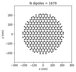
## ----- set up single structure
step = 30
mat = materials.silicon()
geo = structures.nanodisc(step, R=7, H=8, mesh='hex')
struct = structures.struct(step, geo, mat)
struct = structures.center_struct(struct, which_axis=['x','y','z'])


## ----- illumination
wavelengths = np.linspace(1000,1600, 31)
field_generator = fields.plane_wave
field_kwargs = [
    dict(E_s=0, E_p=1, inc_angle=180, inc_plane='xz'), # lin-pol X; normal incidence from below
    dict(E_s=1, E_p=0, inc_angle=135, inc_plane='xz'), # lin-pol Y; normal incidence from below
    ]
efield = fields.efield(field_generator, wavelengths=wavelengths, kwargs=copy.deepcopy(field_kwargs))


## ----- environment: vacuum
n1 = 1.0
dyads = propagators.DyadsQuasistatic123(n1)


## ----- simulation1
sim = core.simulation(struct=struct, efield=efield, dyads=dyads)
visu.structure(sim, tit='N dipoles = {}'.format(len(sim.struct.geometry)))

structure initialization - automatic mesh detection: hex
structure initialization - consistency check: 1679/1679 dipoles valid

/home/pwiecha/.local/lib/python3.8/site-packages/pyGDM2/visu.py:49: UserWarning: 3D data. Falling back to XY projection...
  warnings.warn("3D data. Falling back to XY projection...")

<matplotlib.collections.PathCollection at 0x7f1be6f74280>

## launch full sim for comparison
sim.scatter(method=method)

timing for wl=1000.00nm - setup: EE 1318.8ms, inv.: 931.7ms, repropa.: 416.8ms (2 field configs), tot: 2733.9ms
timing for wl=1020.00nm - setup: EE 58.7ms, inv.: 226.1ms, repropa.: 69.3ms (2 field configs), tot: 361.8ms
timing for wl=1040.00nm - setup: EE 63.7ms, inv.: 222.4ms, repropa.: 70.6ms (2 field configs), tot: 364.2ms
timing for wl=1060.00nm - setup: EE 60.3ms, inv.: 222.3ms, repropa.: 70.8ms (2 field configs), tot: 360.9ms
timing for wl=1080.00nm - setup: EE 58.4ms, inv.: 220.7ms, repropa.: 70.9ms (2 field configs), tot: 357.1ms
timing for wl=1100.00nm - setup: EE 58.8ms, inv.: 220.5ms, repropa.: 70.8ms (2 field configs), tot: 357.3ms
timing for wl=1120.00nm - setup: EE 59.6ms, inv.: 224.5ms, repropa.: 70.5ms (2 field configs), tot: 362.2ms
timing for wl=1140.00nm - setup: EE 58.2ms, inv.: 222.0ms, repropa.: 69.7ms (2 field configs), tot: 358.0ms
timing for wl=1160.00nm - setup: EE 58.9ms, inv.: 221.9ms, repropa.: 70.9ms (2 field configs), tot: 359.5ms
timing for wl=1180.00nm - setup: EE 59.6ms, inv.: 221.7ms, repropa.: 71.6ms (2 field configs), tot: 360.5ms
timing for wl=1200.00nm - setup: EE 60.2ms, inv.: 220.1ms, repropa.: 70.8ms (2 field configs), tot: 358.3ms
timing for wl=1220.00nm - setup: EE 57.8ms, inv.: 221.1ms, repropa.: 70.1ms (2 field configs), tot: 356.6ms
timing for wl=1240.00nm - setup: EE 60.0ms, inv.: 222.7ms, repropa.: 71.1ms (2 field configs), tot: 361.4ms
timing for wl=1260.00nm - setup: EE 64.6ms, inv.: 225.3ms, repropa.: 70.7ms (2 field configs), tot: 368.4ms
timing for wl=1280.00nm - setup: EE 60.7ms, inv.: 222.0ms, repropa.: 70.8ms (2 field configs), tot: 360.8ms
timing for wl=1300.00nm - setup: EE 62.3ms, inv.: 224.3ms, repropa.: 71.6ms (2 field configs), tot: 365.9ms
timing for wl=1320.00nm - setup: EE 67.7ms, inv.: 223.5ms, repropa.: 71.3ms (2 field configs), tot: 370.2ms
timing for wl=1340.00nm - setup: EE 68.1ms, inv.: 220.5ms, repropa.: 71.3ms (2 field configs), tot: 367.0ms
timing for wl=1360.00nm - setup: EE 58.3ms, inv.: 221.2ms, repropa.: 71.5ms (2 field configs), tot: 358.5ms
timing for wl=1380.00nm - setup: EE 61.5ms, inv.: 223.8ms, repropa.: 71.6ms (2 field configs), tot: 364.0ms
timing for wl=1400.00nm - setup: EE 60.4ms, inv.: 221.8ms, repropa.: 70.6ms (2 field configs), tot: 359.7ms
timing for wl=1420.00nm - setup: EE 60.5ms, inv.: 224.6ms, repropa.: 71.2ms (2 field configs), tot: 364.1ms
timing for wl=1440.00nm - setup: EE 63.6ms, inv.: 228.0ms, repropa.: 70.9ms (2 field configs), tot: 369.7ms
timing for wl=1460.00nm - setup: EE 60.9ms, inv.: 221.5ms, repropa.: 70.6ms (2 field configs), tot: 360.1ms
timing for wl=1480.00nm - setup: EE 61.1ms, inv.: 226.6ms, repropa.: 71.0ms (2 field configs), tot: 366.6ms
timing for wl=1500.00nm - setup: EE 59.4ms, inv.: 223.4ms, repropa.: 70.7ms (2 field configs), tot: 361.3ms
timing for wl=1520.00nm - setup: EE 59.9ms, inv.: 224.9ms, repropa.: 70.7ms (2 field configs), tot: 363.4ms
timing for wl=1540.00nm - setup: EE 60.7ms, inv.: 226.4ms, repropa.: 70.6ms (2 field configs), tot: 365.8ms
timing for wl=1560.00nm - setup: EE 61.2ms, inv.: 223.8ms, repropa.: 71.7ms (2 field configs), tot: 364.3ms
timing for wl=1580.00nm - setup: EE 60.8ms, inv.: 239.3ms, repropa.: 71.7ms (2 field configs), tot: 379.0ms
timing for wl=1600.00nm - setup: EE 59.6ms, inv.: 223.3ms, repropa.: 70.4ms (2 field configs), tot: 361.0ms

1

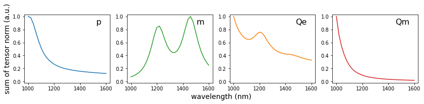
spectral density of modes

Now we calculate spectra of the maximum possible radiated energy of every multipole. This corresponds to integrating the euklidian norm of all generalized polarizability tenors for each multipole and taking it to the power 2.

wls, d_mode_spec = tools.calculate_spectrum(sim, 0, multipole.density_of_multipolar_modes,
                                           which_moments=['p', 'm', 'qe', 'qm'], method=method)

K_E_spec = d_mode_spec.T[0]
K_M_spec = d_mode_spec.T[1]
K_QE_spec = d_mode_spec.T[2]
K_QM_spec = d_mode_spec.T[3]



plt.figure(figsize=(14,2.5))

plt.subplot(141)
plt.title('p', x=0.9, y=0.9, fontsize=16, color='k', ha='right', va='top')
plt.plot(wls, np.array(K_E_spec)/np.max(K_E_spec), color='C0', label='p')
plt.ylabel('sum of tensor norm (a.u.)', fontsize=14)
plt.ylim(-0.02, 1.03)

plt.subplot(142)
plt.title('m', x=0.9, y=0.9, fontsize=16, color='k', ha='right', va='top')
plt.plot(wls, np.array(K_M_spec)/np.max(K_M_spec), color='C2', label='m')
plt.xlabel('wavelength (nm)', x=1.1, fontsize=14)
plt.ylim(-0.02, 1.03)

plt.subplot(143)
plt.title('Qe', x=0.9, y=0.9, fontsize=16, color='k', ha='right', va='top')
plt.plot(wls, np.array(K_QE_spec)/np.max(K_QE_spec), color='C1', label='Qm')
plt.ylim(-0.02, 1.03)

plt.subplot(144)
plt.title('Qm', x=0.9, y=0.9, fontsize=16, color='k', ha='right', va='top')
plt.plot(wls, np.array(K_QM_spec)/np.max(K_QM_spec), color='C3', label='Qe')
plt.ylim(-0.02, 1.03)

plt.show()

wl=1000.0nm. calc. K: 368.0ms.  electric... 12019.0ms.  magnetic... 1678.7ms. Done.
wl=1020.0nm. calc. K: 384.1ms.  electric... 11977.8ms.  magnetic... 1651.1ms. Done.
wl=1040.0nm. calc. K: 386.0ms.  electric... 11781.4ms.  magnetic... 1636.4ms. Done.
wl=1060.0nm. calc. K: 391.2ms.  electric... 11977.5ms.  magnetic... 1652.5ms. Done.
wl=1080.0nm. calc. K: 394.2ms.  electric... 11815.5ms.  magnetic... 1642.3ms. Done.
wl=1100.0nm. calc. K: 409.7ms.  electric... 11983.6ms.  magnetic... 1655.0ms. Done.
wl=1120.0nm. calc. K: 395.6ms.  electric... 11840.1ms.  magnetic... 1650.0ms. Done.
wl=1140.0nm. calc. K: 384.0ms.  electric... 11771.4ms.  magnetic... 1632.8ms. Done.
wl=1160.0nm. calc. K: 401.9ms.  electric... 11856.2ms.  magnetic... 1661.7ms. Done.
wl=1180.0nm. calc. K: 378.2ms.  electric... 11860.4ms.  magnetic... 1644.3ms. Done.
wl=1200.0nm. calc. K: 397.9ms.  electric... 11862.2ms.  magnetic... 1652.1ms. Done.
wl=1220.0nm. calc. K: 397.4ms.  electric... 11898.0ms.  magnetic... 1652.9ms. Done.
wl=1240.0nm. calc. K: 409.4ms.  electric... 11874.9ms.  magnetic... 1663.5ms. Done.
wl=1260.0nm. calc. K: 388.8ms.  electric... 12014.2ms.  magnetic... 1653.8ms. Done.
wl=1280.0nm. calc. K: 389.5ms.  electric... 11858.1ms.  magnetic... 1648.7ms. Done.
wl=1300.0nm. calc. K: 376.7ms.  electric... 11865.9ms.  magnetic... 1650.7ms. Done.
wl=1320.0nm. calc. K: 396.4ms.  electric... 11872.6ms.  magnetic... 1645.0ms. Done.
wl=1340.0nm. calc. K: 394.8ms.  electric... 11979.0ms.  magnetic... 1673.9ms. Done.
wl=1360.0nm. calc. K: 392.3ms.  electric... 12015.6ms.  magnetic... 1663.4ms. Done.
wl=1380.0nm. calc. K: 386.0ms.  electric... 11948.7ms.  magnetic... 1665.4ms. Done.
wl=1400.0nm. calc. K: 395.4ms.  electric... 12006.2ms.  magnetic... 1652.6ms. Done.
wl=1420.0nm. calc. K: 390.3ms.  electric... 11987.1ms.  magnetic... 1668.1ms. Done.
wl=1440.0nm. calc. K: 391.2ms.  electric... 11979.5ms.  magnetic... 1620.2ms. Done.
wl=1460.0nm. calc. K: 405.5ms.  electric... 11845.7ms.  magnetic... 1643.9ms. Done.
wl=1480.0nm. calc. K: 397.9ms.  electric... 11880.5ms.  magnetic... 1648.1ms. Done.
wl=1500.0nm. calc. K: 395.9ms.  electric... 11819.1ms.  magnetic... 1649.2ms. Done.
wl=1520.0nm. calc. K: 399.5ms.  electric... 11865.4ms.  magnetic... 1647.8ms. Done.
wl=1540.0nm. calc. K: 398.7ms.  electric... 11916.7ms.  magnetic... 1650.4ms. Done.
wl=1560.0nm. calc. K: 395.5ms.  electric... 11888.2ms.  magnetic... 1657.2ms. Done.
wl=1580.0nm. calc. K: 391.8ms.  electric... 11884.3ms.  magnetic... 1652.1ms. Done.
wl=1600.0nm. calc. K: 412.4ms.  electric... 11863.8ms.  magnetic... 1642.7ms. Done.

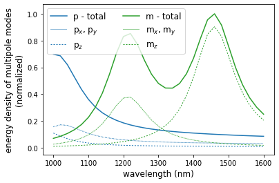
component wise mode density

We can also calculate the maximum possible multipole excitation for each component of the multipole moment.

# =============================================================================
# x/y/z resolved energy density of dipole modes
# =============================================================================
def density_of_m_xyz(sim, field_index=None, wavelength=None, return_mode_energy=True):
    if field_index is not None:
        from pyGDM2 import tools
        wavelength = tools.get_field_indices(sim)[field_index]['wavelength']
    out_list = []

    exp_order = 2 if return_mode_energy else 1
    out_list.append(np.sum(np.linalg.norm(sim.K_M_E[wavelength][:,0,:], axis=(1)))**exp_order)
    out_list.append(np.sum(np.linalg.norm(sim.K_M_E[wavelength][:,1,:], axis=(1)))**exp_order)
    out_list.append(np.sum(np.linalg.norm(sim.K_M_E[wavelength][:,2,:], axis=(1)))**exp_order)

    return np.array(out_list)

def density_of_p_xyz(sim, field_index=None, wavelength=None, return_mode_energy=True):
    if field_index is not None:
        from pyGDM2 import tools
        wavelength = tools.get_field_indices(sim)[field_index]['wavelength']
    out_list = []

    exp_order = 2 if return_mode_energy else 1
    out_list.append(np.sum(np.linalg.norm(sim.K_P_E[wavelength][:,0,:], axis=(1)))**exp_order)
    out_list.append(np.sum(np.linalg.norm(sim.K_P_E[wavelength][:,1,:], axis=(1)))**exp_order)
    out_list.append(np.sum(np.linalg.norm(sim.K_P_E[wavelength][:,2,:], axis=(1)))**exp_order)

    return np.array(out_list)



wl, spec_mmdens = tools.calculate_spectrum(sim, 0, multipole.density_of_multipolar_modes,
                                      which_moments=['p', 'm', 'qe', 'qm'], method=method)
wl, spec_m_d = tools.calculate_spectrum(sim, 0, density_of_m_xyz)
wl, spec_p_d = tools.calculate_spectrum(sim, 0, density_of_p_xyz)

## normalize to maximum of dipole spectra
norm_dp = max([spec_mmdens[:,0].max(), spec_mmdens[:,1].max()])


plt.plot(wl, spec_mmdens[:,0]/norm_dp, color='C0', label='p - total')
plt.plot(wl, spec_p_d[:,0]/norm_dp, color='C0', lw=1, dashes=[1,1], label='p$_x$, p$_y$')
plt.plot(wl, spec_p_d[:,2]/norm_dp, color='C0', lw=1, dashes=[2,2], label='p$_z$')

plt.plot(wl, spec_mmdens[:,1]/norm_dp, color='C2', label='m - total')
plt.plot(wl, spec_m_d[:,0]/norm_dp, color='C2', lw=1, dashes=[1,1], label='m$_x$, m$_y$')
plt.plot(wl, spec_m_d[:,2]/norm_dp, color='C2', lw=1, dashes=[2,2], label='m$_z$')

plt.xlabel("wavelength (nm)", fontsize=12)
plt.ylabel("energy density of multipole modes\n(normalized)", fontsize=12)
plt.legend(fontsize=12, ncol=2)
plt.ylim(-0.05, 1.07)
plt.show()

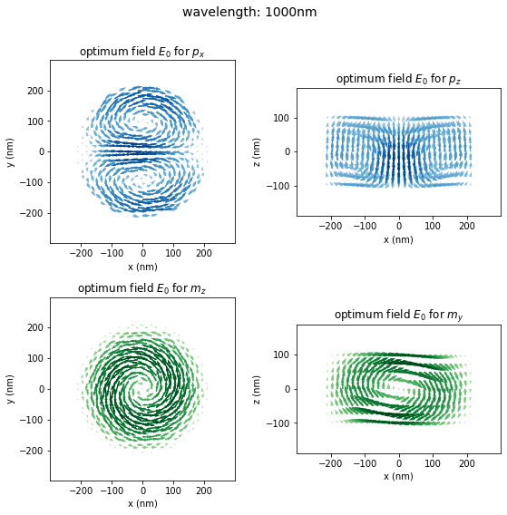
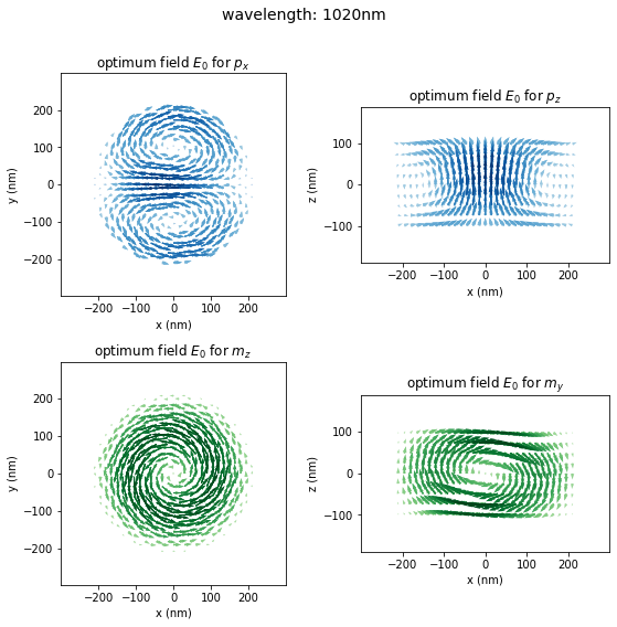
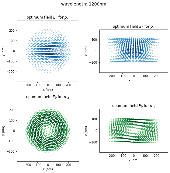
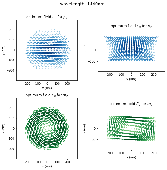
dipole modes: visualize optimum illumination fields

The field required to induce the strongest possible multipole moment is equivalent to the column vectors of the generalized polarizability tensors. Visualization is as simple as selecting the corresponding slice of the numpy array which stores the generalized polarizability:

# =============================================================================
# visualize "optimum" illumination fields
# =============================================================================
test_wavelengths = [1000, 1020, 1200, 1440]

for probe_wl in test_wavelengths:

    KP_opt_field_x = np.concatenate([sim.struct.geometry, sim.K_P_E[probe_wl][:,0,:]], axis=1)
    KP_opt_field_z = np.concatenate([sim.struct.geometry, sim.K_P_E[probe_wl][:,2,:]], axis=1)
    KM_opt_field_y = np.concatenate([sim.struct.geometry, sim.K_M_E[probe_wl][:,1,:]], axis=1)
    KM_opt_field_z = np.concatenate([sim.struct.geometry, sim.K_M_E[probe_wl][:,2,:]], axis=1)

    plt.figure(figsize=(8,8))
    plt.suptitle('wavelength: {}nm'.format(probe_wl), fontsize=14)
    plt.subplot(2,2,1, aspect='equal')
    visu.vectorfield(KP_opt_field_x, show=0, tit='optimum field $E_0$ for $p_x$')
    plt.subplot(2,2,2, aspect='equal')
    visu.vectorfield(KP_opt_field_z, show=0, tit='optimum field $E_0$ for $p_z$', projection='xz')
    plt.subplot(2,2,3, aspect='equal')
    visu.vectorfield(KM_opt_field_z, show=0, tit='optimum field $E_0$ for $m_z$', cmap=plt.cm.Greens)
    plt.subplot(2,2,4, aspect='equal')
    visu.vectorfield(KM_opt_field_y, show=0, tit='optimum field $E_0$ for $m_y$', projection='xz', cmap=plt.cm.Greens)
    plt.tight_layout(rect=(0,0,1,0.97))
    plt.show()

use optimum illumination for new simulation

We can use this field as illumination for a new simulation:

# =============================================================================
# use optimum illumination for new simulation
# =============================================================================
def fixfield(pos, env_dict, wavelength, conf=0, returnField='E', **kwargs):
    """function to use a fixed illumination field for pyGDM2 via a global variable

    Very dirty hack solution. Passing field as function parameter doesn't work
    because of the way in pyGDM2 to hash field indices for spectrum and
    rasterscan calculations.
    """
    global ef_cont
    return ef_cont.ef

class efcontainer():
    __name__='fixfield'
    def __init__(self, ef):
        self.ef = ef


probe_wl = 1020
KP_opt_field = np.concatenate([sim.struct.geometry, sim.K_P_E[probe_wl][:,0,:]], axis=1)

## normalize for use as illumination
KP_opt_field[:,3:] /= np.linalg.norm(KP_opt_field[:,3:], axis=1).max()
ef_cont = efcontainer(KP_opt_field[:,3:])
fieldconf = [dict(conf=0)]

efield_fix = fields.efield(fixfield, wavelengths, fieldconf)
sim_fix = core.simulation(struct, efield=efield_fix, dyads=dyads)
sim_fix.scatter(method=method)

timing for wl=1000.00nm - setup: EE 66.5ms, inv.: 278.9ms, repropa.: 5.5ms (1 field configs), tot: 356.5ms
timing for wl=1020.00nm - setup: EE 64.0ms, inv.: 230.4ms, repropa.: 4.2ms (1 field configs), tot: 304.5ms
timing for wl=1040.00nm - setup: EE 59.8ms, inv.: 233.5ms, repropa.: 4.2ms (1 field configs), tot: 303.7ms
timing for wl=1060.00nm - setup: EE 60.4ms, inv.: 231.4ms, repropa.: 4.3ms (1 field configs), tot: 302.6ms
timing for wl=1080.00nm - setup: EE 58.3ms, inv.: 226.6ms, repropa.: 4.2ms (1 field configs), tot: 295.2ms
timing for wl=1100.00nm - setup: EE 58.3ms, inv.: 229.5ms, repropa.: 4.2ms (1 field configs), tot: 298.3ms
timing for wl=1120.00nm - setup: EE 60.7ms, inv.: 230.9ms, repropa.: 4.2ms (1 field configs), tot: 301.9ms
timing for wl=1140.00nm - setup: EE 58.2ms, inv.: 227.7ms, repropa.: 4.2ms (1 field configs), tot: 296.4ms
timing for wl=1160.00nm - setup: EE 60.8ms, inv.: 234.3ms, repropa.: 4.5ms (1 field configs), tot: 304.7ms
timing for wl=1180.00nm - setup: EE 59.6ms, inv.: 227.6ms, repropa.: 4.2ms (1 field configs), tot: 297.7ms
timing for wl=1200.00nm - setup: EE 61.9ms, inv.: 231.2ms, repropa.: 4.2ms (1 field configs), tot: 303.3ms
timing for wl=1220.00nm - setup: EE 60.9ms, inv.: 232.1ms, repropa.: 4.4ms (1 field configs), tot: 303.5ms
timing for wl=1240.00nm - setup: EE 58.3ms, inv.: 226.3ms, repropa.: 4.2ms (1 field configs), tot: 294.8ms
timing for wl=1260.00nm - setup: EE 58.9ms, inv.: 228.1ms, repropa.: 4.3ms (1 field configs), tot: 297.5ms
timing for wl=1280.00nm - setup: EE 60.1ms, inv.: 229.1ms, repropa.: 4.2ms (1 field configs), tot: 299.7ms
timing for wl=1300.00nm - setup: EE 59.2ms, inv.: 230.3ms, repropa.: 4.3ms (1 field configs), tot: 300.2ms
timing for wl=1320.00nm - setup: EE 58.1ms, inv.: 227.8ms, repropa.: 4.2ms (1 field configs), tot: 297.3ms
timing for wl=1340.00nm - setup: EE 65.1ms, inv.: 231.0ms, repropa.: 4.2ms (1 field configs), tot: 306.3ms
timing for wl=1360.00nm - setup: EE 60.3ms, inv.: 228.5ms, repropa.: 4.2ms (1 field configs), tot: 299.1ms
timing for wl=1380.00nm - setup: EE 60.8ms, inv.: 230.1ms, repropa.: 4.2ms (1 field configs), tot: 301.5ms
timing for wl=1400.00nm - setup: EE 64.0ms, inv.: 225.7ms, repropa.: 4.2ms (1 field configs), tot: 299.9ms
timing for wl=1420.00nm - setup: EE 59.1ms, inv.: 228.1ms, repropa.: 4.2ms (1 field configs), tot: 297.8ms
timing for wl=1440.00nm - setup: EE 58.4ms, inv.: 230.3ms, repropa.: 4.2ms (1 field configs), tot: 299.6ms
timing for wl=1460.00nm - setup: EE 58.7ms, inv.: 227.9ms, repropa.: 4.2ms (1 field configs), tot: 297.1ms
timing for wl=1480.00nm - setup: EE 58.7ms, inv.: 231.8ms, repropa.: 4.9ms (1 field configs), tot: 301.9ms
timing for wl=1500.00nm - setup: EE 60.6ms, inv.: 231.1ms, repropa.: 4.3ms (1 field configs), tot: 303.0ms
timing for wl=1520.00nm - setup: EE 59.9ms, inv.: 227.9ms, repropa.: 4.2ms (1 field configs), tot: 298.3ms
timing for wl=1540.00nm - setup: EE 58.3ms, inv.: 228.5ms, repropa.: 4.3ms (1 field configs), tot: 297.3ms
timing for wl=1560.00nm - setup: EE 58.8ms, inv.: 229.2ms, repropa.: 4.3ms (1 field configs), tot: 298.5ms
timing for wl=1580.00nm - setup: EE 61.7ms, inv.: 230.3ms, repropa.: 4.2ms (1 field configs), tot: 302.6ms
timing for wl=1600.00nm - setup: EE 58.6ms, inv.: 229.9ms, repropa.: 4.2ms (1 field configs), tot: 299.4ms

1

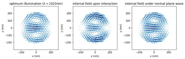
## plot internal fields
plt.figure(figsize=(10,4))

plt.subplot(1,3,1, aspect='equal')
visu.vectorfield(KP_opt_field, show=0, tit='optimum illumination ($\lambda=${}nm)'.format(probe_wl))
plt.subplot(1,3,2, aspect='equal')
fidx_probewl = tools.get_closest_field_index(sim_fix, dict(wavelength=probe_wl))
visu.vectorfield_by_fieldindex(sim_fix, fidx_probewl, show=0, tit='internal field upon interaction')
plt.subplot(1,3,3, aspect='equal')
fidx_probewl = tools.get_closest_field_index(sim, dict(wavelength=probe_wl, E_p=1))
visu.vectorfield_by_fieldindex(sim, fidx_probewl, show=0, tit='internal field under normal plane wave')

plt.tight_layout()
plt.show()

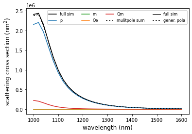
scattering spectra under “ideal” field illumination

This is a conventional pyGDM simulation, so we can calculate for instance scattering spectra (and their multipole decomposition), just as usual.

wls, spec_ex = tools.calculate_spectrum(sim_fix, 0, linear.extinct)
ex, sc, ab = spec_ex.T

wls, mpsc_Kp_spec = tools.calculate_spectrum(sim_fix, 0, multipole.scs, normalization_E0=False)
sc_p_Kp, sc_m_Kp, sc_Qe_Kp, sc_Qm_Kp = mpsc_Kp_spec.T

plt.plot(wls, sc, c='k', label='full sim')
plt.plot(wls, sc_p_Kp, c='C0', label='p')
plt.plot(wls, sc_m_Kp, c='C2', label='m')
plt.plot(wls, sc_Qe_Kp, c='C1', label='Qe')
plt.plot(wls, sc_Qm_Kp, c='C3', label='Qm')
plt.plot(wls, (sc_p_Kp+sc_m_Kp+sc_Qm_Kp+sc_Qe_Kp), c='k', dashes=[2,2], label='mulitpole sum')

plt.plot([], [], c='k', lw=1, label='full sim')
plt.plot([], [], c='k', dashes=[2,2], label='gener. pola')

plt.xlabel('wavelength (nm)', fontsize=12)
plt.ylabel('scattering cross section (nm$^2$)', fontsize=12)
plt.legend(fontsize=8, ncol=4)
plt.show()