Generalized Polarizabilties - Mode density and multiple illuminations
New functionalities in ``multipole`` added in v1.1.3
!!CAUTION!! : ``multipole`` is a new functionality. Please report possible problems and errors.
The generalized polarizabilities (GP) formalism is particularly interesting to calculate the total density of multipole modes of a nanostructure as well as to evaluate rapidly the multipole expansion of the response for various illuminations. How to do this technically is demonstrated in the following.
The GP formalism is based on the exact multipole expansion [1]. It is described in [2].
[1] Alaee, R., Rockstuhl, C. and Fernandez-Corbaton, I. An electromagnetic multipole expansion beyond the long-wavelength approximation. Optics Communications 407, 17-21 (2018)
[2] Majorel et al. Generalized polarizabilites for an exact multipole analysis of complex nanostructures under inhomogeneous illumination. arXiv (2022)
Setup and run simulation
[1]:
from __future__ import print_function, division
import numpy as np
import matplotlib.pyplot as plt
import copy
from pyGDM2 import structures
from pyGDM2 import materials
from pyGDM2 import fields
from pyGDM2 import tools
from pyGDM2 import propagators
from pyGDM2 import linear
from pyGDM2 import core
from pyGDM2 import visu
from pyGDM2 import multipole
# =============================================================================
# sim setup
# =============================================================================
method = 'lu'
#method = 'cupy'
## ----- set up single structure
step = 24
mat = materials.dummy(3.5)
geo = structures.spheroid(step, R1=10, R2=5, R3=5, mesh='hex')
struct = structures.struct(step, geo, mat)
struct = structures.center_struct(struct, which_axis=['x','y','z'])
## ----- illumination
wavelengths = np.linspace(500, 1500, 26)
field_generator = fields.plane_wave
field_kwargs = dict(E_s=0, E_p=1, inc_angle=0, inc_plane='xz') # lin-pol X, normal incidence from below
efield = fields.efield(field_generator, wavelengths=wavelengths, kwargs=copy.deepcopy(field_kwargs))
## ----- environment: vacuum
n1 = 1.0
dyads = propagators.DyadsQuasistatic123(n1)
## ----- simulation1
sim = core.simulation(struct=struct, efield=efield, dyads=dyads)
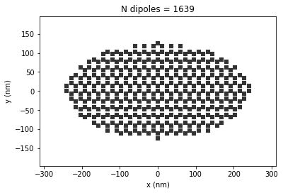
visu.structure(sim, tit='N dipoles = {}'.format(len(sim.struct.geometry)))
structure initialization - automatic mesh detection: hex
structure initialization - consistency check: 1639/1639 dipoles valid
/home/pwiecha/.local/lib/python3.8/site-packages/pyGDM2/visu.py:49: UserWarning: 3D data. Falling back to XY projection...
  warnings.warn("3D data. Falling back to XY projection...")
[1]:
<matplotlib.collections.PathCollection at 0x7fc3b7a9fa90>
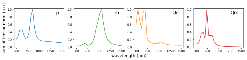
spectral density of modes
Now we calculate spectra of the maximum possible radiated energy of every multipole. This corresponds to integrating the euklidian norm of all generalized polarizability tenors for each multipole and taking it to the power 2.
[2]:
wl, d_mode_spec = tools.calculate_spectrum(
            sim, 0, multipole.density_of_multipolar_modes, method=method,
            which_moments=['p', 'm', 'qe', 'qm'])

K_E_spec = d_mode_spec.T[0]
K_M_spec = d_mode_spec.T[1]
K_QE_spec = d_mode_spec.T[2]
K_QM_spec = d_mode_spec.T[3]


plt.figure(figsize=(14,2.5))

plt.subplot(141)
plt.title('p', x=0.9, y=0.9, fontsize=16, color='k', ha='right', va='top')
plt.plot(wl, np.array(K_E_spec)/np.max(K_E_spec), color='C0', label='p')
plt.ylabel('sum of tensor norm (a.u.)', fontsize=14)
plt.ylim(-0.02, 1.03)

plt.subplot(142)
plt.title('m', x=0.9, y=0.9, fontsize=16, color='k', ha='right', va='top')
plt.plot(wl, np.array(K_M_spec)/np.max(K_M_spec), color='C2', label='m')
plt.xlabel('wavelength (nm)', x=1.1, fontsize=14)
plt.ylim(-0.02, 1.03)

plt.subplot(143)
plt.title('Qe', x=0.9, y=0.9, fontsize=16, color='k', ha='right', va='top')
plt.plot(wl, np.array(K_QE_spec)/np.max(K_QE_spec), color='C1', label='Qm')
plt.ylim(-0.02, 1.03)

plt.subplot(144)
plt.title('Qm', x=0.9, y=0.9, fontsize=16, color='k', ha='right', va='top')
plt.plot(wl, np.array(K_QM_spec)/np.max(K_QM_spec), color='C3', label='Qe')
plt.ylim(-0.02, 1.03)

plt.show()
wl=500.0nm. calc. K: 2285.7ms.  electric... 11505.5ms.  magnetic... 1583.4ms. Done.
wl=540.0nm. calc. K: 334.8ms.  electric... 11359.3ms.  magnetic... 1566.2ms. Done.
wl=580.0nm. calc. K: 334.5ms.  electric... 11334.1ms.  magnetic... 1594.9ms. Done.
wl=620.0nm. calc. K: 335.9ms.  electric... 11187.7ms.  magnetic... 1549.6ms. Done.
wl=660.0nm. calc. K: 334.5ms.  electric... 11185.6ms.  magnetic... 1551.1ms. Done.
wl=700.0nm. calc. K: 331.2ms.  electric... 11280.3ms.  magnetic... 1567.9ms. Done.
wl=740.0nm. calc. K: 340.2ms.  electric... 11302.2ms.  magnetic... 1563.4ms. Done.
wl=780.0nm. calc. K: 339.3ms.  electric... 11294.4ms.  magnetic... 1570.0ms. Done.
wl=820.0nm. calc. K: 324.5ms.  electric... 11276.7ms.  magnetic... 1565.6ms. Done.
wl=860.0nm. calc. K: 336.4ms.  electric... 11375.3ms.  magnetic... 1577.9ms. Done.
wl=900.0nm. calc. K: 327.6ms.  electric... 11200.2ms.  magnetic... 1553.6ms. Done.
wl=940.0nm. calc. K: 338.7ms.  electric... 11295.6ms.  magnetic... 1565.4ms. Done.
wl=980.0nm. calc. K: 314.8ms.  electric... 11299.1ms.  magnetic... 1579.6ms. Done.
wl=1020.0nm. calc. K: 337.5ms.  electric... 11159.4ms.  magnetic... 1547.1ms. Done.
wl=1060.0nm. calc. K: 331.9ms.  electric... 11497.7ms.  magnetic... 1587.5ms. Done.
wl=1100.0nm. calc. K: 341.9ms.  electric... 11344.7ms.  magnetic... 1568.3ms. Done.
wl=1140.0nm. calc. K: 334.0ms.  electric... 11360.8ms.  magnetic... 1577.8ms. Done.
wl=1180.0nm. calc. K: 323.5ms.  electric... 11343.4ms.  magnetic... 1573.1ms. Done.
wl=1220.0nm. calc. K: 322.5ms.  electric... 11363.0ms.  magnetic... 1566.5ms. Done.
wl=1260.0nm. calc. K: 323.0ms.  electric... 11390.7ms.  magnetic... 1593.4ms. Done.
wl=1300.0nm. calc. K: 335.8ms.  electric... 11340.7ms.  magnetic... 1571.2ms. Done.
wl=1340.0nm. calc. K: 339.4ms.  electric... 11367.1ms.  magnetic... 1586.2ms. Done.
wl=1380.0nm. calc. K: 342.5ms.  electric... 11210.0ms.  magnetic... 1551.0ms. Done.
wl=1420.0nm. calc. K: 330.0ms.  electric... 11248.0ms.  magnetic... 1553.0ms. Done.
wl=1460.0nm. calc. K: 343.4ms.  electric... 11356.4ms.  magnetic... 1590.7ms. Done.
wl=1500.0nm. calc. K: 337.9ms.  electric... 11324.0ms.  magnetic... 1566.5ms. Done.
configure various illumination fields
This is done using the normal pyGDM API and in particular its efield class.
[3]:
wavelengths = sim.efield.wavelengths

## ------ plane wave - various incident angles
field_generator = fields.plane_wave
field_kwargs_S = [
    dict(E_s=1, E_p=0, inc_angle=angle, inc_plane='xz')
    for angle in np.linspace(0, 90, 10)
    ]
field_kwargs_P = [
    dict(E_s=0, E_p=1, inc_angle=angle, inc_plane='xz')
    for angle in np.linspace(0, 90, 10)
    ]

efield1 = fields.efield(field_generator, wavelengths=wavelengths, kwargs=field_kwargs_S)
efield2 = fields.efield(field_generator, wavelengths=wavelengths, kwargs=field_kwargs_P)


## ------ dipole illumination, e/m dipole of various orientations
field_generator_p = fields.dipole_electric
field_generator_m = fields.dipole_magnetic
field_kwargs_dp = [
    dict(x0=300, y0=0, z0=0,
         mx=np.sin(angle), my=0, mz=np.cos(angle))
                for angle in np.linspace(-np.pi/2,0, 9)]

efield3 = fields.efield(field_generator_p, wavelengths=wavelengths, kwargs=field_kwargs_dp)
efield4 = fields.efield(field_generator_m, wavelengths=wavelengths, kwargs=field_kwargs_dp)
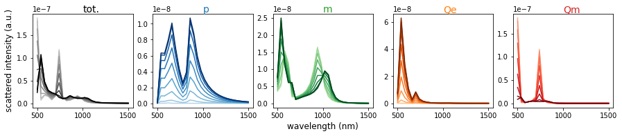
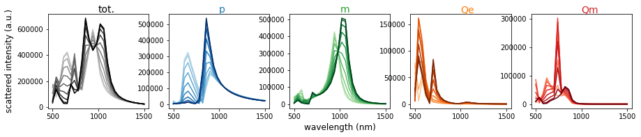
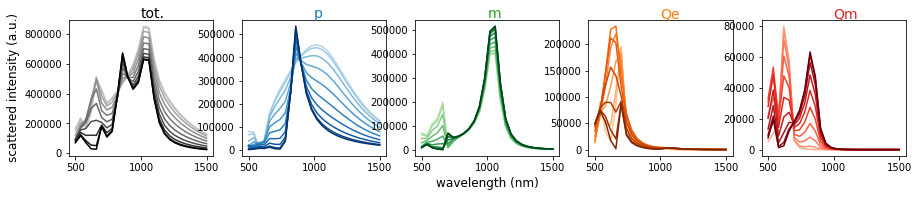
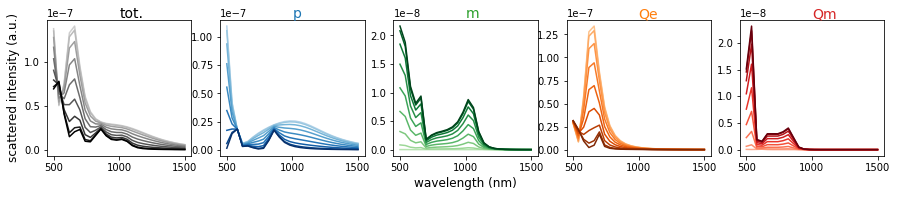
evalute all illumination fields
Now we use the generalized polarizabities to evaluate the multipole expansion of each illumination.
[5]:
for _ef in [efield1, efield2, efield3, efield4]:
    sim.efield = _ef
    all_spec = []
    for i in range(len(tools.get_possible_field_params_spectra(sim))):
        kw = tools.get_possible_field_params_spectra(sim)[i]

        ## calculate spectra using multiprocessing
        wl, mpsc_Kp_spec = tools.calculate_spectrum(sim, i, multipole.scs,
                                use_generalized_polarizabilities=True,
                                normalization_E0=False, N_cpu=16)
        sc_p_Kp, sc_m_Kp, sc_Qe_Kp, sc_Qm_Kp = mpsc_Kp_spec.T
        all_spec.append(mpsc_Kp_spec)
    all_spec = np.array(all_spec)


    print(_ef)

    colors0 = plt.cm.Greys(np.linspace(0.3, 1, len(all_spec)))
    colors1 = plt.cm.Blues(np.linspace(0.3, 1, len(all_spec)))
    colors2 = plt.cm.Greens(np.linspace(0.3, 1, len(all_spec)))
    colors3 = plt.cm.Oranges(np.linspace(0.3, 1, len(all_spec)))
    colors4 = plt.cm.Reds(np.linspace(0.3, 1, len(all_spec)))

    plt.figure(figsize=(15,2.5))
    # ax0 = plt.subplot(161); plt.title('mode density', x=0.5, y=1.05, fontsize=14, color='k', ha='left', va='top')
    ax1 = plt.subplot(151); plt.title('tot.', x=0.5, y=1.05, fontsize=14, color='k', ha='left', va='top')
    ax2 = plt.subplot(152); plt.title('p', x=0.5, y=1.05, fontsize=14, color='C0', ha='left', va='top')
    ax3 = plt.subplot(153); plt.title('m', x=0.5, y=1.05, fontsize=14, color='C2', ha='left', va='top')
    ax4 = plt.subplot(154); plt.title('Qe', x=0.5, y=1.05, fontsize=14, color='C1', ha='left', va='top')
    ax5 = plt.subplot(155); plt.title('Qm', x=0.5, y=1.05, fontsize=14, color='C3', ha='left', va='top')
    for i in range(len(tools.get_possible_field_params_spectra(sim))):
        kw = tools.get_possible_field_params_spectra(sim)[i]

        ax1.plot(wl, np.sum(all_spec[i], axis=-1), color=colors0[i])
        ax2.plot(wl, all_spec[i,:,0], color=colors1[i])
        ax3.plot(wl, all_spec[i,:,1], color=colors2[i])
        ax4.plot(wl, all_spec[i,:,2], color=colors3[i])
        ax5.plot(wl, all_spec[i,:,3], color=colors4[i])

    ax3.set_xlabel('wavelength (nm)', fontsize=12)
    ax1.set_ylabel(r'scattered intensity (a.u.)', fontsize=12)
    plt.show()
 ----- incident field -----
   field generator: "plane_wave"
   26 wavelengths between 500.0 and 1500.0nm
   10 incident field configurations per wavelength
 ----- incident field -----
   field generator: "plane_wave"
   26 wavelengths between 500.0 and 1500.0nm
   10 incident field configurations per wavelength
 ----- incident field -----
   field generator: "dipole_electric"
   26 wavelengths between 500.0 and 1500.0nm
   9 incident field configurations per wavelength
 ----- incident field -----
   field generator: "dipole_magnetic"
   26 wavelengths between 500.0 and 1500.0nm
   9 incident field configurations per wavelength