Tutorial: Multi-material and graded structures

01/2021: updated to pyGDM v1.1+

This tutorial demonstrates how to create nanostructures composed of multiple materials or with a graded refractive index.

Load modules

import numpy as np
import matplotlib.pyplot as plt

from pyGDM2 import structures
from pyGDM2 import materials
from pyGDM2 import fields
from pyGDM2 import propagators

from pyGDM2 import core
from pyGDM2 import visu
from pyGDM2 import tools
from pyGDM2 import linear

Gold-Silicon-Gold sandwich structure

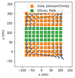
Instead of defining the dispersion as a single instance of a material class, it is possible to assing a material to every meshpoint of the nanostructure. To do so, we create a list of material class instances, each element corresponds to the material of the according element in the geometry list.

Here we create 3 blocks (each 10x3x4 meshpoints), the first and the last are gold blocks, and in their center we will stack a silicon block.

## --------------- Setup structure
mesh = 'cube'
step = 20.0

## block 1: gold
geom1 = structures.rect_wire(step, L=10,H=3,W=4, mesh=mesh)
mat1 = len(geom1)*[materials.gold()]

## block 2: silicon. Move Y by width of block1
geom2 = structures.rect_wire(step, L=10,H=3,W=4, mesh=mesh)
geom2.T[1] += 4*step
mat2 = len(geom2)*[materials.silicon()]

## block 3: gold. Move Y by widths of block1 and block2
geom3 = structures.rect_wire(step, L=10,H=3,W=4, mesh=mesh)
geom3.T[1] += 8*step
mat3 = len(geom3)*[materials.gold()]


## put together the two blocks (list of coordinate AND list of materials)
geometry = np.concatenate([geom1, geom2, geom3])
material = mat1 + mat2 + mat3

Now we wrap it in the struct object and create the usual simulation object with a plane wave illumination.

## structure instance
struct = structures.struct(step, geometry, material)


## incident field
field_generator = fields.planewave
kwargs = dict(theta=0)
wavelengths = [500]
efield = fields.efield(field_generator, wavelengths=wavelengths, kwargs=kwargs)

## environment
n1, n2 = 1.0, 1.0  # vacuum
dyads = propagators.DyadsQuasistatic123(n1=n1, n2=n2)

## simulation initialization
sim = core.simulation(struct, efield, dyads)


## --------------- run scatter simulation
sim.scatter(verbose=True)


## ------------- plot
## plot geometry and real-part of E-field
visu.structure(sim, show=0)
visu.vectorfield_by_fieldindex(sim, 0)

structure initialization - automatic mesh detection: cube
structure initialization - consistency check: 360/360 dipoles valid

/home/hans/.local/lib/python3.8/site-packages/numba/core/dispatcher.py:237: UserWarning: Numba extension module 'numba_scipy' failed to load due to 'ValueError(No function '__pyx_fuse_0pdtr' found in __pyx_capi__ of 'scipy.special.cython_special')'.
  entrypoints.init_all()

timing for wl=500.00nm - setup: EE 3002.9ms, inv.: 203.6ms, repropa.: 800.5ms (1 field configs), tot: 4007.8ms

/home/hans/.local/lib/python3.8/site-packages/pyGDM2/visu.py:49: UserWarning: 3D data. Falling back to XY projection...
  warnings.warn("3D data. Falling back to XY projection...")

<matplotlib.quiver.Quiver at 0x7fb2878f5250>

We run the simulation and plot the structure and the electric field vectors (realp part) in the XY plane. Note that the visualization function visu.struct recongized the different materials and colors by default the corresponding parts of the structure.

Structure with graded refractive index

In a second example, we will create a structure with graded refractive index. To do so, we just loop over all discretization elements and define the according material based on the spatial position of the meshpoint.

## ------------- Setup structure
mesh = 'cube'
step = 20.0
geo = structures.rect_wire(step, L=40, H=5, W=5, mesh=mesh)

## graded material, refindex increasing from 1 to 4 (from left to right)
material = []
value_for_plotting = []
for pos in geo:
    ## grade from 1.0 to 4.0
    n = 1.0 + 3*(pos[0] - geo.T[0].min()) / (geo.T[0].max()-geo.T[0].min())
    material.append(materials.dummy(n))
    value_for_plotting.append(n)              # helper list for plotting of index grading

struct = structures.struct(step, geo, material)


## incident field
field_generator = fields.planewave        # planwave excitation
kwargs = dict(theta = [90])              # several polarizations
wavelengths = [500]                     # one single wavelength
efield = fields.efield(field_generator, wavelengths=wavelengths, kwargs=kwargs)


## simulation initialization, use same environment as above
sim = core.simulation(struct, efield, dyads)

structure initialization - automatic mesh detection: cube
structure initialization - consistency check: 1000/1000 dipoles valid

Run simulation and plot

## ------------- run scatter simulation
efield = core.scatter(sim, verbose=True)



## ------------- plot
## plot geometry and real-part of E-field
sc = plt.scatter(geo.T[0], geo.T[1], c=value_for_plotting)
plt.colorbar(sc, label="refractive index")
visu.vectorfield_by_fieldindex(sim, 0, tit='electric field vector inside (real part)')

## nearfield 2 steps above structure
r_probe = tools.generate_NF_map(-600,600,101, -600,600,101, Z0=geo.T[2].max()+2*step)
Es, Et, Bs, Bt = linear.nearfield(sim, 0, r_probe)

visu.structure_contour(sim, color='w', show=0)
im = visu.vectorfield_color(Es, tit='intenstiy of scattered field outside', show=0)
plt.colorbar(im, label=r'$|E_s|^2 / |E_0|^2$')
plt.show()

timing for wl=500.00nm - setup: EE 140.2ms, inv.: 1050.5ms, repropa.: 10.1ms (1 field configs), tot: 1201.4ms

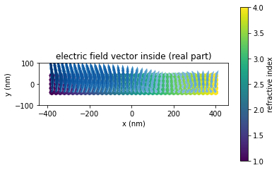
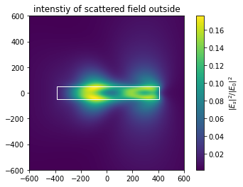
In the grading loop above, we added the refractive index to a second list value_for_plotting, which we now used to plot the refractive index of the structure on a color-scale together with the electric field vectors (real part) inside the structure (top plot).

For the bottom plot, we calculated the scattered electric field intensity 2 stepsizes above the structure.