Tutorial: Visualize the indicent field

01/2021: updated to pyGDM v1.1+

In this quick tutorial we demonstrate how to visualize fundamental fields without any structure (hence no simulation is done here).

We first load some modules

import matplotlib.pyplot as plt

from pyGDM2 import fields
from pyGDM2 import tools
from pyGDM2 import visu

The field generator

We will use an p-polarized, oblique incident plane wave, which is partially reflected at a thin metallic layer on a thick glass substrate with vacuum above. First we setup the environment to pass to the field generator:

field_generator = fields.plane_wave

## in the new API pyGDM v1.1+, the field-generators take as input the positions
## to evaluate the field at, the wavelength and a dictionary "env_dict" which
## contains informations about the environment.
## The parameters depend on the field-generator and need to be also
## supported by the `Dyads` class which is used in combination with the
## field generator. So far all generators and classes support a 3-layer system
## with two semi-infinite layers sourrounding a center medium of finite thickness.
## The supported `env_dict` entries can be found in the documentation of the
## respective field-generator functions.

## --- layered environment
n3 = 1.0            # vacuum
n2 = 1.05 + 1.8j    # lossy interface layer (metallic)
n1 = 1.5            # dielectric substrate
spacing = 40.0      # thickness of interface layer `n2` (in nm)

env_dict = dict(eps1=n1**2, eps2=n2**2, eps3=n3**2, spacing=spacing)

Setup the test frame and evaluate the field

Now we need to setup the test-frame. We use a thin metallic layer (lossy), sandwiched between glass and vacuum. We want to plot the field in the XZ plane.

## --- 2D evaluation plane
projection = 'XZ'
r_probe = tools.generate_NF_map(-500,500,30, -400,600,30,0, projection=projection)

## --- evaluation of the field-generator
wavelength = 500
NF = field_generator(r_probe, env_dict, wavelength,
                     inc_angle=45, E_s=0, E_p=1)

Plot the result of the field-generator

## -- helper function to plot the interface layer
def plot_layer():
    plt.axhline(0, color='w',lw=1); plt.axhline(0, dashes=[2,2], color='k',lw=1)
    plt.axhspan(0,spacing, color='k', ls='--', fc='orange', alpha=0.35)
    plt.axhline(spacing, color='w',lw=1); plt.axhline(spacing, dashes=[2,2], color='k',lw=1)
    plt.arrow(350, -350, -150, 150, head_width=50, head_length=80, fc='k', ec='k')




plt.figure(figsize=(12,5))
plt.subplot(141, aspect='equal')
v = visu.vectorfield(NF, r_probe, complex_part='real', projection=projection, tit=projection+' real part', show=0)
plot_layer()

plt.subplot(142, aspect='equal')
v = visu.vectorfield(NF, r_probe, complex_part='imag', cmap=plt.cm.Reds, projection=projection, tit=projection+' imag part',  show=0)
plot_layer()


plt.subplot(243, aspect='equal')
v = visu.vectorfield_color(NF, r_probe, projection=projection, tit='intensity: '+r'$|E|^2/|E0|^2$', show=0)
plt.colorbar(v)
plt.xticks([]); plt.yticks([])
plot_layer()

plt.subplot(244, aspect='equal')
v = visu.vectorfield_color(NF, r_probe, projection=projection, fieldComp='ex', tit='Ex', show=0)
plt.colorbar(v)
plt.xticks([]); plt.yticks([])
plot_layer()

plt.subplot(247, aspect='equal')
v = visu.vectorfield_color(NF, r_probe, projection=projection, fieldComp='ey', tit='Ey', show=0)
plt.colorbar(v)
plt.xticks([]); plt.yticks([])
plot_layer()

plt.subplot(248, aspect='equal')
v = visu.vectorfield_color(NF, r_probe, projection=projection, fieldComp='ez', tit='Ez', show=0)
plt.colorbar(v)
plt.xticks([]); plt.yticks([])
plot_layer()

plt.show()

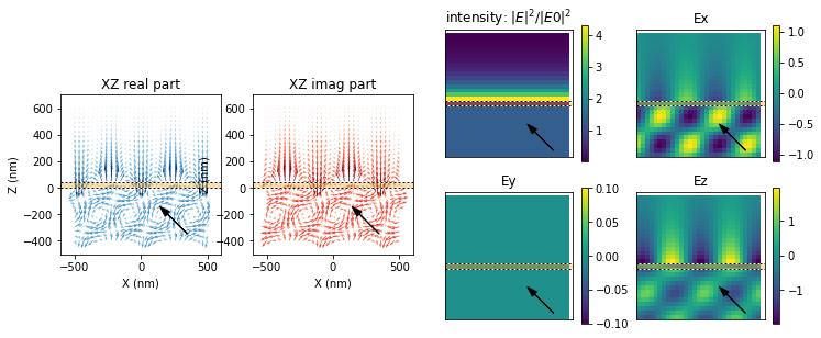
Note: The black arrow indicates the direction and angle of incidence of the plane wave.